• View
• Edit
• History
• Print

Combinatorial Alternative to Wave Function, Derivation Of The Classification Of ShefferPolynomials, 20230109 Research Program Fivesome, Outgrowths

Double Causality: A Framework for Physics

I am rewriting this overview. I am preparing slides that along with this page will be the basis for a new video overviewing this research. I will state what I have learned so far and what questions I am exploring further. This includes my related research priorities.

I need to provide combinatiorial interpretations of the following:

• The definition of the Hermite polynomials. (Done)
• The recursion relation for the Hermite polynomials. (Done)
• The orthogonality relation for the Hermite polynomials. (I need to undertand the paper by Kim and Zeng.)
• The Hamiltonian operator's action on the Hermite polynomial. (I need to interpret the action and also translate from physicist Hermite polynomials to probabilist Hermite polynomials.)

The x's (free space, position) are time events that stay fixed. The i's (momentum) are time events that switch order (they link two events, two interactions). What does it mean if we switch from position to momentum, if we take the Fourier transform?

---

• Summary
• Goals and Ingredients
• Cognitive Framework: Fivesome
• Combinatorial Interpretation of Schroedinger's equation
• Sheffer polynomials
• Orthogonal Sheffer polynomials
• Combinatorial interpretation
• Space-time wrapper
• Scattering Zones
• Wick's theorem
• Feynman diagrams
• Space-time
• Calculating observables
• Overview of combinatorial interpretation
• Links to papers
• Related pages

Hypothesis to explore

• Physical solutions to the Schroedinger equation, and their analogues in quantum field theory, are precisely those established by orthogonal Sheffer polynomials, and the physics can be comprehended through their combinatorics.

Three inspirations

• Hermite and Laguerre polynomials appear in solutions of the Schroedinger equation for the quantum harmonic oscillator and the radial component of the hydrogen atom, respectively.
• My PhD in algebraic combinatorics with skills for interpreting the meaning of such algebraic expressions, how they define combinatorial objects and act on them. And my belief that nature has something to say!
• My appreciation for a fivefold cognitive framework whereby "every effect has had its cause; but not every cause had had its effects; so there is a critical point for deciding".

Want to find a combinatorial interpretation for the measurement of the Hamiltonian {$\hat{H}$} given a wave function {$\psi$}

{$\langle H\rangle =\int\psi^*\hat{H}\psi dx = \langle\psi | \hat{H}\psi\rangle $}

where, for example, {$\psi_n(x) = D_n\textrm{He}_n(\sqrt{\frac{2m\omega}{\hbar}}x) e^{-\frac{m\omega}{2\hbar}x^2}$}

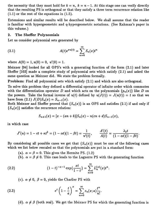
We are given the generating function for the orthogonal Sheffer polynomials {$P_n(x)$}.

{$\sum_{n=0}^{\infty}P_n(x)\frac{t^n}{n!}=A(t)e^{xu(t)}$}

I write the recurrence relation as follows:

{$P_{n+1}(x)=[x-(ln+f)]P_n(x)-[kn(n-1)-\gamma n]P_{n-1}(x)$}

Combinatorially, we will see that the coefficients in the recurrence relation are weights for combinatorial components:

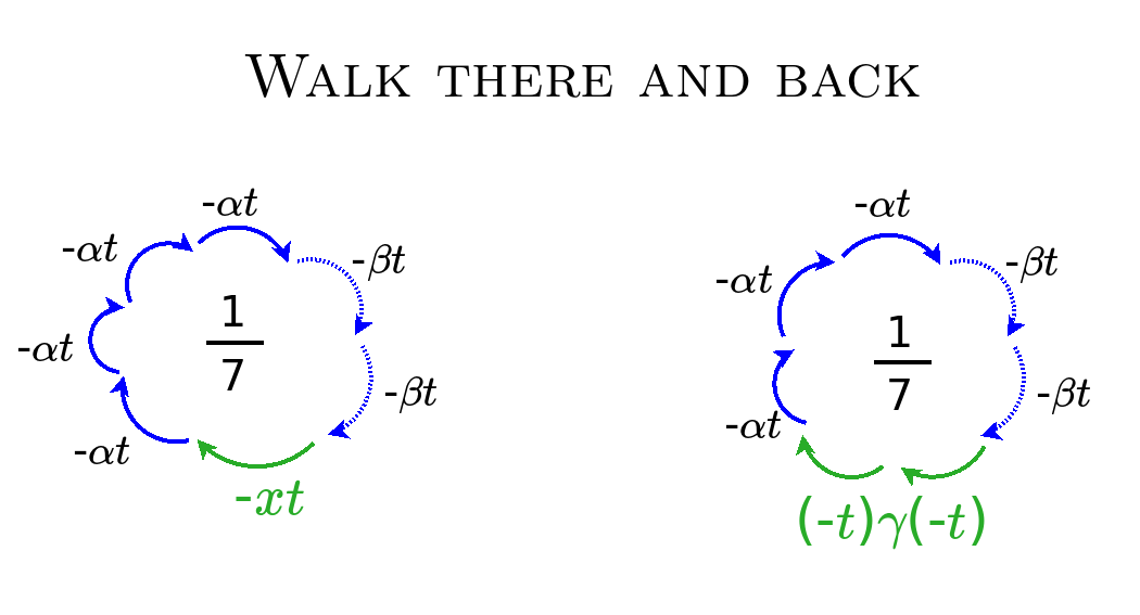
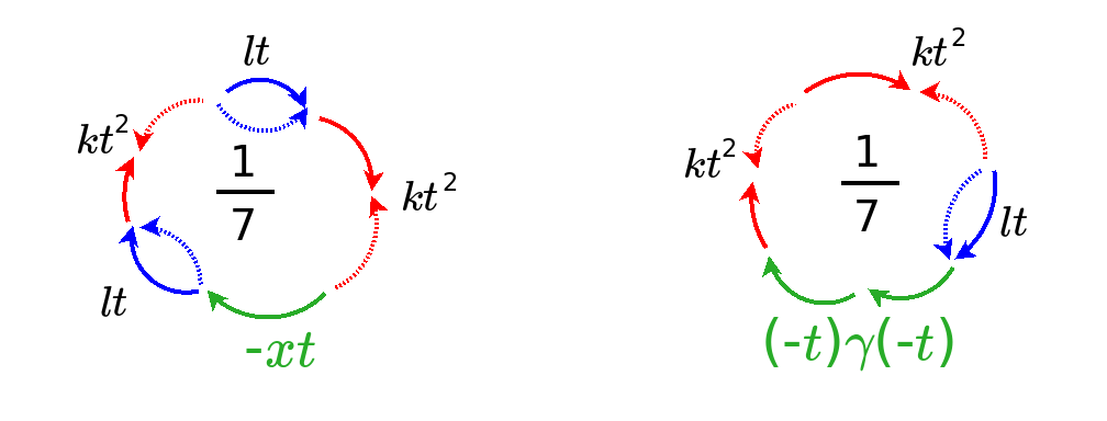
• {$l=(-\alpha)+(-\beta)$} causal (one-step) link in a causal tree
• {$k=(-\alpha)(-\beta)$} causal (two-step) kink in a causal tree
• {$f$} causal tree with a single root (also signifying a translation in x)
• {$\gamma$} cycle

The weights {$\alpha$} and {$\beta$} are the basis for the fivefold classification. We have {$(\alpha-\beta)^2=l^2-4k$}.

{$\alpha,\beta = \frac{\alpha + \beta}{2}\pm \frac{\alpha - \beta}{2} = -\frac{l}{2}\pm\frac{\sqrt{l^2-4k}}{2}$}

{$u'(t)=\frac{1}{(1-\alpha t)(1-\beta t)} = \frac{1}{1 + lt + kt^2} = \frac{A'(t)}{\gamma t A(t)} = \frac{1}{\gamma t}\frac{\textrm{d}}{\textrm{dt}}\textrm{ln}A(t)$}

{$u'(t)=1+t(\alpha + \beta)+t^2(\alpha^2+\alpha\beta+\beta^2)+\cdots$} interpreted as particle clocks

{$u'(t)= \frac{1}{\alpha-\beta}[(\alpha - \beta) + (\alpha^2 - \beta^2)t + (\alpha^3-\beta^3)t^2 + \cdots]$}

{$u(t)=t+\frac{1}{2}t^2(\alpha + \beta)+\frac{1}{3}t^3(\alpha^2+\alpha\beta+\beta^2)+\cdots$} has an extra point in each circle which is placed and then removed (how does that relate to quantum perturbation?)

The constraint of orthogonality yields the constraint {$A(t)=e^{\gamma v(t)}$} where

{$v(t)=\frac{1}{2}t^2 + \frac{1}{3}t^3(\alpha + \beta)+\frac{1}{4}t^4(\alpha^2+\alpha\beta+\beta^2)+\cdots $} has an extra double point in each circle which is placed and then removed

{$v'(t) = t +t^2(\alpha + \beta)+t^3(\alpha^2+\alpha\beta+\beta^2)+\cdots$}

{$v'(t)=tu'(t)$} is the quantum perturbation of {$u(t)$}.

{$A(t)=e^{\gamma (\frac{1}{2}t^2 + \frac{1}{3}t^3(\alpha + \beta)+\frac{1}{4}t^4(\alpha^2+\alpha\beta+\beta^2)+\cdots)}$}

Thus {$\sum_{n=0}^{\infty}P_n(x)\frac{t^n}{n!}=e^{\gamma v(t)+xu(t)}$}

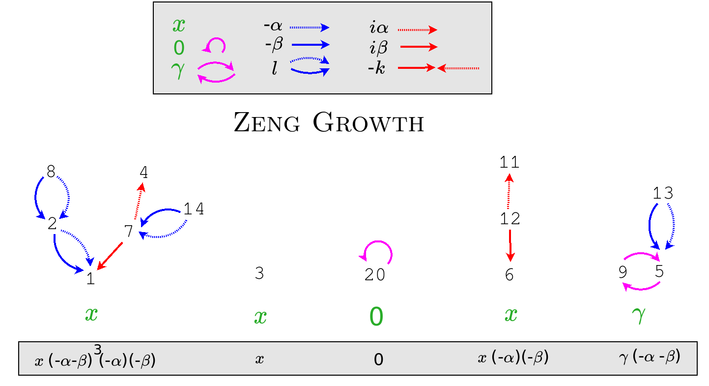
{$\mathcal{L}[x^n]=\sum_{\sigma\in S_n}\alpha^{\textrm{asc}(\sigma)}\beta^{\textrm{desc}(\sigma)}(\frac{f}{\alpha\beta})^{\textrm{fix}(\sigma)}(\frac{-\gamma}{\alpha\beta})^{\textrm{cyc}(\sigma)-\textrm{fix}(\sigma)}$}

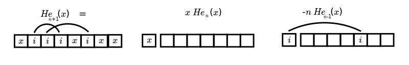
{$\frac{\textrm{d}}{\textrm{dx}}\textrm{He}_n(x) = n\textrm{He}_{n-1}(x)$}

{$x\textrm{He}_n(x) = \textrm{He}_{n+1}(x) + n\textrm{He}_{n-1}(x)$} because {$\textrm{He}_{n+1}(x) = x\textrm{He}_n(x) - n\textrm{He}_{n-1}(x)$}

{$t(u(s))=s$}

{$t(D)=D+t_2D^2+t_3D^3+\cdots$}

{$t(D)P_n(x)=nP_{n-1}(x)$}

{$t(D)=\frac{e^{(\alpha-\beta)D}-1}{e^{(\alpha-\beta)D}-\beta}$}

Mathematically, specifically, I want to:

• Understand how to derive the classification of orthogonal Sheffer polynomials.
• Interpret combinatorially the coefficients of these polynomials.
• Interpret combinatorially the equation {$\sum_{n=0}^{\infty}P_n(x)=A(t)e^{xu(t)}$}
• Interpret combinatorially the recurrence relation.

---

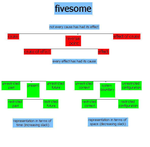
The fivesome refers to the division of everything into five perspectives, that which is needed for decision making, and which yield two representations, one in terms of time and the other in terms of space.

Here are two presentations that I gave about the fivesome:

• Time and Space as Representations of Decision-Making
• Consciousness as the Social Awareness Schema of a Disembodying Mind

The main idea of this conceptual framework: Every effect has had its cause. Not every cause has had its effect.

• Our minds can move backwards from effect to cause, but also forwards from cause to effect. And a fifth perspective (the present or the boundary) relates the two causal directions.

We conceive this framework by way of two conceptions, in terms of time and in terms of space.

• In time, the cause is in the past, the effect is in the future, and the present relates them in both directions.
• In space, the cause is outside of a system, the effect is inside of a system, and a boundary separates them.

Examples of double causality

• Jesus offers communion. "He took bread, and when he had given thanks, he broke and gave it to them, saying, 'This is my body which is given for you. Do this in memory of me.'"
• Bob Dylan, "Don't think twice". "I wish that there was something you could do or say to try and make me change my mind and stay but we never did too much talking, anyway, so don't think twice, it's all right."
• Beatles, "She loves you". "You think you've lost your love. Well, I saw her yesterday. It's you she's thinking of and she told me what to say. She say's she loves you."
• Beatles, "Yesterday". "Yesterday love was such an easy game to play. Now I need a place to hide away. Oh, I believe in yesterday."
• John Lennon, "God". "I don't believe in Jesus, ... I don't believe in Zimmerman, I don't believe in Beatles. I just believe in me Yoko and me. And that's reality. The dream is over. What can I say? The dream is over. Yesterday. I was the dream weaver, but now I'm reborn. I was the Walrus, but now I'm John. And so dear friends, you'll just have to carry on. The dream is over."

{$i\hbar\frac{\partial\Psi}{\partial t}=-\frac{\hbar^2}{2m}\frac{\partial^2\Psi}{\partial x^2}+V\Psi$}

{$i\hbar\frac{\partial\Psi}{\partial t} + \frac{\hbar^2}{2m}\frac{\partial^2\Psi}{\partial x^2}=V\Psi$}

Solutions of Schroedinger's equation are orthogonal Sheffer polynomials

• A wave function which is a solution to Schroedinger's equation can be thought of as consisting of an orthogonal polynomial (the information state) and a weight function (the space-time wrapper).
• Question to investigate: In what sense can I claim that the only mathematical solutions to Schroedinger's equation are those which have this form?
• Question to investigate: Are there examples of mathematical solutions or physical solutions that do not have this form?
• Solutions for the quantum harmonic oscillator are based on Hermite polynomials, and solutions for the hydrogen atom are based on Laguerre polynomials.
• These are orthogonal polynomials and their weight functions provide the inner product that is the basis for the Schroedinger equation.
• The orthogonal polynomials and weight function depend on the potential specified.
• Question to investigate: Assuming the solutions are orthogonal polynomials, then what are the possible potentials?

{$\langle Q\rangle =\int\Psi^*\hat{Q}\Psi \textrm{dx}=\langle\Psi |\hat{Q}\Psi\rangle$}

A combinatorial interpretation of a physical observable relates three elements.

• The equation is satisfied by orthogonal polynomials.
  • Their coefficients are integers that have combinatorial interpretations.
  • The polynomials are in terms of a variable (such as x) which can be given a combinatorial interpretation (such as cells of free space).
• Orthogonality is expressed with regard to a weight function that can be thought of as a space-time wrapper.
  • The combinatorics can be interpreted in terms of the moments, thus bypassing the wrapper, the sum or integral.
  • However, the weight function can also be interpreted combinatorially.
• The physical operator, the observable, can be interpreted as a shift of orthogonal polynomials, by way of the relevant Rodrigues' formula, which is then multiplied with the conjugates of the originals and then submitted to the orthogonality relations.

Working hypothesis: In physical situations, the orthogonal polynomials must be Sheffer polynomials.

• When other polynomials occur, such as Chebyshev polynomials for the infinite well, then we only get toy models which do not actually occur in physics.

Question to investigate: What is special about Sheffer polynomials?

• How are Sheffer polynomials related to Lie theory?

answered by Tom Copeland, Shadows of Simplicity

Hidden structure, hidden symmetry, that is waiting to be discovered.

• Maxwell's theory of the electromagnetic field, as we know, contains two hidden symmetries that will rock twentieth century physics. One is relativistic invariance and the other is gauge invariance. Now, both of these symmetries were already contained in Maxwell's theory, but nobody including Maxwell in the 19th century noticed it. And so is it conceivable that our present day theory also contains some kind of hidden structure? To me, that's a possibility. Hidden structure that's waiting for young people to discover just like Einstein discovered relativistic invariance hidden in Maxwell's equation and Hermann Weyl discovers gauge invariance in Maxwell's theory. – Anthony Zee, October 14, 2020, Quantum Field Theory: An Overview, 29:15.

---

Sheffer polynomial sequences {$\{P_n(x)\}$} are those with respect to which the shift operator {$T_a$} commutes with the operator Q. The shift operator is defined by {$T_af(x)=f(x+a)$}, and the operator Q is defined by {$QP_n(x)=nP_{n-1}(x)$}. The operator Q acts like a derivative on the highest power, and the remaining terms can be thought of as echo terms, which are dependent on the highest power of each polynomial in the sequence. Thus we have {$(T_aQ-QT_a)P_n(x)=0$}.

Sheffer sequences form a group under the operation of umbral composition, which is defined as follows. Given polynomial sequences {$p_n(x)=\sum_{k=0}^{n=\infty}a_{n,k}x^k$} and {$q_n(x)=\sum_{k=0}^{n=\infty}b_{n,k}x^k$}, we define the {$n$}th term of {$p\circ q$} as {$(p_n\circ q)(x)=\sum_{k=0}^na_{n,k}q_k(x)x^k=\sum_{n\geq k>l\geq 0}a_{n,k}b_{k,l}x^l$}. [Investigation: Interpret this combinatorially.]

A scanned copy of an important article, Some properties of polynomial sets of type zero by I.M.Sheffer, Duke Mathematical Journal, September 1939, pages 590-622, is available here through Archive.org It also available to subscribers here through Project Euclid.

Sheffer polynomials {$\{P_n(x)\}$} have the form {$\sum_{n=0}^{\infty}P_n(x)t^n=A(t)e^{xu(t)}$}.

It is helpful to construct a generating sequence {$J(y)$}, a formal inverse to {$u(t)$}, such that {$J(u(t)) = u(J(t)) = t$}.

{$u(t)=\sum_{k=1}^{\infty}u_kt^k=t+u_2t^2+u_3t^3+\cdots$}

{$J(y)=\sum_{l=1}^{\infty}j_ly^l=y+j_2y^2+j_3y^3+\cdots$}

{$J(u(t))=\sum_{l=1}^{\infty}j_l(\sum_{k=1}^{\infty}u_kt^k)^l$}

{$u(J(t))=\sum_{k=1}^{\infty}u_k(\sum_{l=1}^{\infty}j_lt^l)^k$}

By examining {$J(u(t)) = u(J(t)) = t$} fo-r each power {$t$}, e can get {$j_l$} in terms of the {$u_k$} and vice versa.

{$j_1=u_1=1$}

{$j_2+u_2=0$} thus {$j_2=-u_2$}

{$j_3+2j_2u_2+u_3=0$} thus {$j_3=-u_3+2u_2^2$}

{$j_4+ 2j_3u_2 +2j_2u_3 +j_2^2u_2 +j_2u_2^2 + 3j_3u_3 + u_4 = 0$} thus {$j_4=-u_4 + 3u_3^2 - 6u_2^2u_3 - 4u_2^3 + 4u_2u_3$}

Note that the equations are symmetric in {$j$} and {$u$}.

{$\frac{\textrm{d}}{\textrm{dt}}J(u(t))=\frac{\textrm{d}}{\textrm{dt}}t=1$}

{$\frac{\textrm{dJ}}{\textrm{du}}\frac{\textrm{du}}{\textrm{dt}}=1$}

{$J'(u)\equiv\frac{\textrm{dJ}}{\textrm{du}}=\frac{1}{u'(t)}$}

Let {$D=\frac{\textrm{d}}{\textrm{dx}}$}.

{$$DA(t)e^{xu(t)}=A(t)(u(t))e^{xu(t)}$$}

{$$D^kA(t)e^{xu(t)}=A(t)(u(t))^ke^{xu(t)}$$}

{$$J(D)A(t)e^{xu(t)}=\sum_{k=1}^{\infty}j_kA(t)(u(t))^ke^{xu(t)}$$}

{$$=A(t)e^{xu(t)}\sum_{k=1}^{\infty}j_k(u(t))^k$$}

{$$=A(t)e^{xu(t)}J(u(t))$$}

{$$=A(t)e^{xu(t)}t$$}

{$$J(D)\sum_{n=0}^{\infty}P_n(x)t^n = \sum_{n=0}^{\infty}P_n(x)t^{n+1}$$}

By considering the coefficient for {$t^n$} we see that {$J(D)P_n(x)=P_{n-1}(x)$}.

---

All orthogonal polynomials satisfy a recurrence relation of the form {$xP_n(x) = P_{n+1}(x) + A_n P_n(x) + B_n P_{n-1}(x)$}.

More specifically, Sheffer polynomials satisfy a recurrence relation written by various authors as follows:

• Meixner per Butzer and Koornwinder: {$P_{n+1}(x)=[x+(l_1+n\lambda)]P_n(x)+[n(k_2+(n-1)\kappa]P_{n-1}(x)$}
• Kim and Zeng: {$P_{n+1}(x)=[x-(\alpha\beta + nu_3+nu_4)]P_n(x)-[n(\beta + n-1)u_1u_2]P_{n-1}(x)$}
  • Equivalently: {$P_{n+1}(x)=[x - (u_3+u_4)n + \alpha\beta)]P_n(x)-[u_1u_2n(n-1) + u_1u_2\beta n]P_{n-1}(x)$}

I will write it in the following form to emphasize the combinatorial meaning of the terms

{$P_{n+1}(x)=[x-(ln+cf)]P_n(x)-[kn(n-1)+cn]P_{n-1}(x)$}

Combinatorially, we will see that the variables are weights for components:

• {$l$} causal (one-step) link
• {$k$} causal (two-step) kink
• {$f$} "free" root of a tree (also signifying a translation in x)
• {$\gamma$} cycle

We can assume that {$f$} = 0 because that's equivalent to translating {$x$} to {$x-f$}.

We will be expressing the weights in terms of {$\alpha$} and {$\beta$}. Notably {$l=(-\alpha)+(-\beta)$} and {$k=(-\alpha)(-\beta)$}. This yields a discriminant

{$$A'(t) = - c f t + \textrm{echo terms}$$}

(where elsewhere I write {$-\gamma = -cf$})(Or is this {$A(t)$}?)

{$$u'(t) = 1 - lt + (l^2-k)t^2 + \textrm{echo terms}$$}

I mean by "echo terms" that the higher order terms are completely determined by the initial terms and have no independent significance.

The following paper has a helpful exposition for calculating {$u(t)$} and {$A(t)$}.

Given the recurrence relation

{$P_{n+1}(x)=(x+\lambda_{n+1})P_n(x) - \mu_{n+1}P_{n-1}(x)$}

And given {$\sum_{n=0}^{\infty}P_n(x)t^n = A(t)e^{xu(t)}$}, where {$A(t)=\sum_{n=0}^{\infty}a_nt^n$} and {$u(t)=\sum_{n=0}^{\infty}u_nt^n$} we multiply out

{$$\sum_{n=0}^{\infty}P_n(x)t^n = \sum_{k_0=0}^{\infty}a_{k_0}t^{k_0}\cdot\sum_{k_1=0}^{\infty}\frac{(xt)^{k_1}}{k_1!}\cdot\sum_{k_2=0}^{\infty}\frac{(u_2xt^2)^{k_2}}{k_2!}\cdot\sum_{k_3=0}^{\infty}\frac{(u_3xt^3)^{k_3}}{k_3!}\cdots$$}

We can use this to calculate, for each polynomial {$P_n(x)=\sum_{k=0}^nP_{n,k}x^k$} it's highest order terms, by looking in the expansion above for the term {$t^nx^{n-s}$} where {$s=0,1,2,\dots$}. We get two linear Diophantine equations {$k_1 + k_2 + k_3 + \cdots = n-s$} and {$k_0+k_1+2k_2+3k_3+\cdots$} and given {$n$} and {$s$} we look for nonnegative solutions.

This allows us to figure out the higher orders terms for {$P_{n+1}(x), P_n(x), P_{n-1}(x)$}. Then, using the recurrence relation, we can conclude that {$\lambda_{n+1}$} is at most linear in {$n$} and {$\mu_{n+1}$} is at most quadratic in {$n$} as follows.

{$\lambda_{n+1}=a_1+2h_2n$}

{$\mu_{n+1}=(a_1^2 - 2a_2 + 2a_1h_2-4h_2^2+3h_3)n + (4h_2^2-3h_3)n^2$}

We solve {$a_1+2h_2n = -(-\alpha - \beta)n - cf$} yielding

{$a_1=-cf, h_2=\frac{\alpha + \beta}{2}$}

We solve {$(a_1^2 - 2a_2 + 2a_1h_2-4h_2^2+3h_3)n + (4h_2^2-3h_3)n^2 = \alpha\beta n(n-1)+nc = \alpha\beta n^2 + n(c-\alpha\beta)$}

This yields {$h_3=\frac{1}{3}(\alpha^2 + \alpha\beta + \beta^2)$} and {$a_2=\frac{1}{2}[c^2f^2 - cf(\alpha + \beta) - c]$}

Calculating {$u(t)$}

I am trying to relate the notation in Sheffer with that in Kim & Zeng.

Sheffer calls {$H(t)$} what I am writing {$u(t)$}.

He sets {$ u'(t)=\sum_{n=0}^{\infty}q_{n+1,1}t^n$}. Thus {$u^{(k)}(0)=(k-1)!q_{k,1}$}. But I know that {$u^{(k)}(0) = (k-1)!(\alpha^{k-1}+\alpha^{k-2}\beta + \cdots + \alpha\beta^{k-2}+\beta^{k-1})$}. Thus {$q_{k,1} = \alpha^{k-1}+\alpha^{k-2}\beta + \cdots + \alpha\beta^{k-2}+\beta^{k-1} $}.

Calculating {$A(t)$}

Using Sheffer's notation...

Define {$\frac{A'(t)}{A(t)} = \sum_{k=0}^{\infty}q_{k+1,0}t^k $}.

{$$\frac{\textrm{d}}{\textrm{dt}}\textrm{ln}A(t)=\frac{A'(t)}{A(t)}$$}

{$$ \textrm{ln}A(t) = \int\sum_{k=0}^{\infty}t^k\textrm{dt} = \sum_{k=0}^{\infty}\int t^k\textrm{dt} = \sum_{k=0}^{\infty}\frac{q_{k+1,0}}{k+1}t^{k+1} $$}

{$$ A(t) = e^{\sum_{k=0}^{\infty}\frac{q_{k+1,0}}{k+1}t^{k+1}} = e^{q_{1,0}t + \frac{1}{2}q_{2,0}t^2 + \frac{1}{3}q_{3,0}t^3 + \cdots} $$}

{$$ A(t) = 1 + (q_{1,0}t + \frac{1}{2}q_{2,0}t^2 + \frac{1}{3}q_{3,0}t^3 + \cdots) + \frac{1}{2}(q_{1,0}t + \frac{1}{2}q_{2,0}t^2 + \frac{1}{3}q_{3,0}t^3 + \cdots)^2 + \frac{1}{6}(q_{1,0}t + \frac{1}{2}q_{2,0}t^2 + \frac{1}{3}q_{3,0}t^3 + \cdots)^3 + \cdots $$}

{$$ A(t) = 1 + t(q_{1,0}) + t^2(\frac{1}{2}q_{2,0} + \frac{1}{2}q_{1,0}^2) + t^3(\frac{1}{3}q_{3,0} + \frac{1}{2}q_{1,0}q_{2,0} + \frac{1}{6}q_{1,0}^3) + \cdots $$}

Recurrence relation

Sheffer gives the recurrence relation, in his notation: {$q_{k+2,1} = \gamma q_{k+1,1} + \epsilon q_{k,1}$}

Here {$\gamma = \alpha + \beta = - (-\alpha - \beta)$} and {$\epsilon = - \alpha\beta = - (-\alpha)(-\beta) $} in my notation.

The recurrence relation yields the characteristic equation {$u^2 = \gamma u + \epsilon $}. This equation expresses the ansatz that solutions will have the form {$q_{k,1} = r^n$}. This equation yields three outcomes, see the article Linear recurrence with constant coefficients.

• If the characteristic equation has two distinct real roots, then the general solutions are as follows: {$a_{n}=C\lambda _{1}^{n}+D\lambda _{2}^{n}$}
• If the two roots are identical, then the general solutions are: {$a_{n}=C\lambda ^{n}+Dn\lambda ^{n}$}
• If the two roots are complex conjugates, then ...

Relating {$P_n(x)$}, {$u(t)$} and {$A(t)$}

From Sheffer:

{${P'}_n(x)=u_1P_{n-1}(x) + u_2P_{n-2}(x) + \cdots + u_nP_0(x)$}

As Sheffer notes, this equation shows that {$u(t)$} by itself determines {${P'}_n(x)$}. Thus {$A(t)$} simply contributes the constant term that must be determined in integrating {${P'}_n(x)$} to yield {$P_n(x)$}. In the form

{$nP_n(x)=\sum_{k=1}^{\infty}(q_{k,0}+xq_{k,1})P_{n-k}$} where {$\frac{A'(t)}{A(t)}=\sum_{k=0}^{\infty}q_{k+1,0}t^k$} and {$u'(t)=\sum_{k=0}^{\infty}q_{k,0}t^k$}

it is apparent that {$A(t)$} contributes the constant terms and {$u(t)$} contributes the coefficients of {$x$}.

Interpreting {$u(t)$} and {$A(t)$}

We can choose to write

{$$u'(t) = \frac{1}{(1-\alpha t)(1-\beta t)} = 1 + (\alpha + \beta) t + (\alpha^2 + \alpha\beta + \beta^2)t^2 + \textrm{echo terms}$$} {$$=(1+\alpha t+\alpha^2t^2+...)(1+\beta t+\beta^2t^2+...) = \sum_{n=0}^{\infty}t^n\sum_{i=0}^n \alpha^i\beta^{n-i}$$}

We have {$l=(-\alpha)+(-\beta)$} and {$k=(-\alpha)(-\beta)$} and {$(1-\alpha t)(1-\beta t) = 1+lt+kt^2$}. And we have, comparing our notation and Meixner's notation, {$-c=k_2$}. Thus we have

{$$u'(t)=\frac{1}{(1-\alpha t)(1-\beta t)}=\frac{1}{1+lt+kt^2}=\frac{A'(t)}{-ctA(t)}$$}

In the most general case, the solution gives the Meixner polynomials.

{$u(t)$}	{$\textrm{ln}A(t)$}	{$A(t)$}	{$e^{x(u(t))}$}
{$\frac{1}{\beta - \alpha}\textrm{ln}(1-\alpha t)+\frac{1}{\alpha - \beta}\textrm{ln}(1-\beta t)$}	{$\frac{\gamma}{\alpha \beta}[\frac{\alpha}{\alpha - \beta} \textrm{ln}(1-\beta t) - \frac{\beta}{\alpha - \beta} \textrm{ln}(1 - \alpha t)]$}	{$(\frac{(1-\beta t)^\alpha}{(1-\alpha t)^\beta})^{\frac{\gamma}{\alpha\beta(\alpha - \beta)}}$}	{$(\frac{1-\beta t}{1-\alpha t})^{\frac{x}{\alpha-\beta}}$}

Fivefold classification

Various specializations of the Meixner polynomials yield a fivefold classification.

polynomials	{$\alpha$}, {$\beta$}	{$u'(t)$}	{$u(t)$}
Meixner	{$\alpha \neq \beta$}, both real, nonzero	{$\frac{1}{(1-\alpha t)(1-\beta t)}$}	{$\frac{1}{\beta - \alpha}\textrm{ln}(1-\alpha t)+\frac{1}{\alpha - \beta}\textrm{ln}(1-\beta t)$}
Charlier	{$\alpha\neq\beta$}, {$\beta=0$}	{$\frac{1}{1-\alpha t}$}	{$-\frac{1}{\alpha}\textrm{ln}(1-\alpha t)$}
Laguerre	{$\alpha=\beta$}, {$\beta\neq 0$}	{$\frac{1}{(1-\alpha t)^2}$}	{$\frac{t}{(1 - \alpha t)}$}
Hermite	{$\alpha=\beta$}, {$\beta=0$}	{$1$}	{$t$}
Meixner-Pollaczek	{$\alpha=\overline{\beta}$}, complex conjugates, nonzero	{$\frac{1}{(1-\alpha t)(1-\overline{\alpha} t)}$}	{$\frac{1}{\overline{\alpha} - \alpha}\textrm{ln}(1-\alpha t)+\frac{1}{\alpha - \overline{\alpha}}\textrm{ln}(1-\overline{\alpha} t)$}

Technically, it is important to express the polynomials in a notation which makes it possible to compare them as participants in a unified quantum narrative. Here is my notation.

I write the recurrence relation:

• {$P_{n+1}(x)=[x-(ln+cf)]P_n(x)-[kn(n-1) + nc]P_{n-1}(x)$}
• {$P_{n+1}(x)=[x-((-\alpha)+(-\beta))n+cf)]P_n(x)-[(-\alpha)(-\beta)n(n-1) + nc]P_{n-1}(x)$}

Meixner polynomials

• Historically, the Meixner polynomials {$m_n(x;\beta,c)$} are not written in monic form. In my notation, the Meixner polynomials are:
  • {$m_n(x;\frac{c}{\alpha\beta},\frac{\alpha}{\beta})=\frac{1}{\alpha^n}P_n((\alpha-\beta)x)$}
  • {$\frac{\alpha}{\beta}m_{n+1}(x)=[\frac{\alpha -\beta}{\beta}x + \frac{\alpha + \beta}{\beta}n+\frac{c}{\beta}(1-\frac{\alpha}{\beta})]m_n(x) - [n(n-1) + n\frac{c}{\alpha\beta}]m_{n-1}(x)$}
  • {$m_{n+1}(x)=\frac{1}{\alpha}[\alpha(n + (x-c)) + \beta(n - x) + c]m_n(x) - \frac{\beta}{\alpha}[n(n-1) + n\frac{c}{\alpha\beta}]m_{n-1}(x)$}
• But we need them in monic form. In my notation, nothing changes and we simply have the recurrence relation for the general case, except with the added condition that {$\alpha-\beta=1$}, which we get by solving for {$\alpha$} and {$\beta$} in terms of {$c$}.

The Sheffer family satisfies the recurrence relation below, with initial polynomials {$P_{-1}=0$} and {$P_0=1$}:

{$$P_{n+1}(x) = (x - (nl + f)) P_n(x) - n(nk + c) P_{n-1}(x)$$}

Writing it like this helps remember that {$l$} is the weight for links, {$k$} for kinks, {$f$} for fixed points (self-entangled trees), {$\gamma$} for cycles (trees). Here {$x$} is taken without coefficient and so the resulting polynomials are all monic. A coefficient can always be introduced by substituting {$x=\gamma y$}. {$f$} is trivial in that it corresponds to a translation of {$x$} and thus can be set as zero.

---

---

---

Space-time wrapper

Each orthogonal polynomial has a corresponding weight function against which it is integrated against. The weight function serves as the inner product with regard to which it is orthogonal.

Polynomial	Weight {$w(x)$}	Combinatorial interpretation
Meixner	step function {$\frac{a^k(\beta)_k}{k!}$} on interval {$[k,k+1)$}
Charlier	step function {$\frac{a^k}{k!}$} on interval {$[k,k+1)$}
Laguerre	{$x^\alpha e^{-x}$}	Tracy-Widom distribution upper end, weak coupling, lower temperature, particles
Hermite	{$e^{-x^2}$}	Tracy-Widom distribution lower end, strong coupling, higher temperature, plasma
Meixner-Pollaczek	{$\frac{|\Gamma(\frac{n+ix}{2})|^2}{|\Gamma(\frac{n}{2})|^2}e^{-x\;\textrm{tan}^{-1}\delta} $}

The {$k$}th moment {$\mu_k$} of an orthogonal polynomial is gotten by integrating {$x^k$} against the weight {$\textrm{dw}$}.

{$$\mu_k=\int x^k \textrm{dw}$$}

In the case of the various Sheffer polynomials, these moments are fundamental numbers in combinatorics which count the most basic objects.

See also: Corteel, Kim, Stanton. Moments of Orthogonal Polynomials and Combinatorics.

Relate these to the construction of families of Zeng trees or of cycle double paths.

Polynomial	Moment {$\mu_n$}	Combinatorial interpretation	Abstract data structure	Possibility functions {$a_k,q_k,s_k$}	{$L(x^n)$}	Example when n=4
Meixner	ordered Bell number	ordered set partitions of n (weak orderings)(made of links)	linear list	{$k+1,0,k$}		541 in all: W>X>Y>Z, W>X>Y=Z, W>X=Y>Z, W>X=Y=Z, W=X>Y>Z ... Y>X>W>Z ... Y=Z>X=W etc.>
Charlier	Bell number {$B_n$}	set partitions of n (equivalence relations)	symbol table	{$k+1,k,1$}		15 in all: {1}{2}{3}{4}, {12}{3}{4}, {13}{2}{4}, {14}{2}{3}, {23}{1}{4}, {24}{1}{2}, {34}{1}{2},{12}{34},{13}{24},{14}{23},{123}{4},{124}{3},{134}{2},{234}{1},{1234}.
Laguerre	n!	permutations of n (strict orderings)	dictionary	{$k+1,2k+1,k$}		24 in all: 1234=(), 1243=(34), 1324=(23), 1342=(234), 1423=(243), 1432=(24), 2134=(12), 2143=(12)(34), 2314=(123), etc.
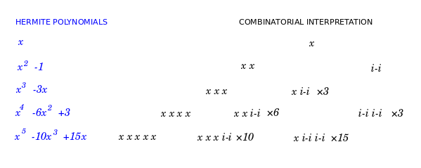
Hermite	(n-1)!! or 0	permutations of n where each cycle is disjoint and has length 2	priority queue	{$k+1,0,1$}		3 in all: (12)(34), (13)(24), (14)(23)
Meixner-Pollaczek	Secant number {$A_{2n}$}	zig zag permutations of 2n (like kinks)				61 in all: 1 < 3 > 2 < 4 > 6 < 8 > 7 and 2 < 6 > 3 < 8 > 1 < 7 > 4 < 5 etc.

Kim and Zeng have a general formula for the moment, which in our case specializes to

{$$L(x^n)=\sum_{\sigma\in S_n}(-\alpha)^{a\sigma} (-\beta)^{d\sigma} 0^{fix\sigma}(\frac{-\gamma}{\alpha\beta})^{cycle\sigma}$$}

Thus the moment {$\mu_n$} considers permutations of length n, where the steps {$\alpha$} indicate ascents, steps {$\beta$} indicate descents, and the translation steps {$f$} (if we had {$f\neq 0$}), would indicate fixed points. (Evidently, fixed points of permutations characterize translations in Minkowski space.)

Narrative of the moments

I need to consider Kim and Zeng's general formula for the moment in terms of a narrative by which the combinatorial object changes. They can all be related to permutations of length n with ascents and descents indicated. There is a process of forgetting:

• Moments of Meixner polynomials yield ordered set partitions. With the arisal of the wave function, we forget the order.
• Moments of Charlier polynonmials yield set partitions. With a bound state we forget ...? and have permutations.
• Moments of Laguerre polynomials yield permutations.
• Moments of Hermite polynomials yield involutions... because every permutation can be considered a pair of involutions?
• Moments of Meixner-Pollaczek polynomials yield alternating permutations... because... ?

Describe these narrative moves as functors. And look for an adjunction relating the moments with the distributions. This should yield an adjoint string.

Sylvie Corteel, Jang Soo Kim, Dennis Stanton. Moments of Orthogonal Polynomials and Combinatorics. describes how, given the recurrence relation, we can calculate the polynomials and the moments. This is the basis for the combinatorial interpretation in terms of Favard paths (for the polynomials) and Motzkin paths (for the moments).

Sylvie Corteel, Jang Soo Kim, Dennis Stanton. Moments of Orthogonal Polynomials and Combinatorics. provides these formulas.

The Hankel determinant {$\Delta_n$} is defined in terms of the moments {$\{\mu_n\}$}.

{$\Delta_n=\begin{pmatrix} \mu_0 & \mu_1 & \dots & \mu_n\\ \mu_1 & \mu_2 & \dots & \mu_{n+1}\\ \vdots & \vdots & \ddots & \vdots\\ \mu_{n} & \mu_{n+1} & \dots & \mu_{2n} \end{pmatrix}$}

The monic polynomial {$P_n(x)$} is given from the moments by

{$P_n(x) = \frac{1}{\Delta_{n-1}}\begin{vmatrix} \mu_0 & \mu_1 & \dots & \mu_n\\ \mu_1 & \mu_2 & \dots & \mu_{n+1}\\ \vdots & \vdots & \ddots & \vdots\\ \mu_{n-1} & \mu_{n} & \dots & \mu_{2n-1} \\ 1 & x & \dots & x^n \end{vmatrix}$}

Quantum Field Theory

The Schroedinger equation is only a preliminary model of quantum reality. We need to add special relativity and we also need to allow for the ongoing creation and annihilation of particles. Thus we need to consider quantum field theory.

The Invisible Bowling Ball

Modify the classical picture of fast moving marbles scattering off a bowling ball.

Think of the "interaction potential" as an invisible bowling ball, the sum of the relevant quantum fields.

If we suppose that the field drops off further away, for example, as {$\frac{1}{r^2}$}, then at a large enough distance, by the Heisenberg uncertainty principle, the field becomes too subtle to be meaningful in any way. Thus we can say that at a certain distance it does not exist, but then at a certain distance it does.

The two roots {$\{{\alpha, \beta}\}$} describe the particle's clock. The clock can be thought of as relating two coordinate systems by steps {$\alpha$} from one to the other and by steps {$\beta$} going back. The steps can be thought of as ticks by the clock. Setting {$\alpha$} and {$\beta$} equal synchronizes the clocks. Setting {$\alpha$} or {$\beta$} to {$0$} resets the clock.

There are 5 zones:

• {$\{{\alpha, \beta}\}$} - distant past, asymptotically free - unentangled state
• {$\{{\alpha, 0}\}$} - entering the interaction potential - wave packet
• {$\{{\alpha, \alpha}\}$} - within the interaction potential - bound state
• {$\{{0, 0}\}$} - leaving the interaction potential - free space
• {$\{\alpha, \bar{\alpha}\}$} - distant future, asymptotically free - entangled state

Remarks

• Currently, as far as I know, quantum field theory only considers the zone where particles are leaving the interaction potential. This is akin to free space.
• In what sense do the clocks themselves establish Minkowski space-time? What need, if any, do we have for a continuum of space-time?
• Starting with Feynman diagrams (the lowest layer of the QFT theoretical cake) work backwards with alternate versions of Wick's theorem corresponding to each of the five zones. What does this yield in place of the traditional quantum field theory (the Hermite case)?
• All of physics should be understood in terms of pairs of reference frames which are related by particle clocks.

Understanding the 5 zones in terms of an event

Reference frame with step {$\beta$} measures with regard to the entering of an event and reference frame with step {$\alpha$} measures with regard to the leaving of an event.

• Before the interaction, the particle clock has steps that are real and independent, {$\{{\alpha, \beta}\}$}, which express the grid from the perspective of the two reference frames.
• Reference frame with step {$\beta$} enters the event and resets itself to zero so we have {$\{{\alpha, 0}\}$} while the other frame continues counting as before.
• Then the reset frame (in the event) now counts along {$\beta = \alpha$} with the frame which has yet to leave the event. This is the bound state, {$\{{\alpha, \alpha}\}$}.
• Then the frame with step {$\alpha$} leaves the event and resets itself to zero, and so they are both zero, as they were both equal: {$\{{0, 0}\}$}
• Then the two frames are counting as conjugates {$\{\alpha, \bar{\alpha}\}$} where the real component is the same and the imaginary component is opposite.

What happens if we reverse time and enter the event from the opposite direction? What happens to nonentanglement and entanglement?

Initial state and final state

Creation and annihilation operators

Creation and annihilation operators, Ladder operator

{$a\mid\! n\rangle= \sqrt{n} \ |n-1\rangle$}

The eigenvalue {$sqrt{n}$} of the annihilation operator is based on the state {$n$} it is leaving.

{$a^\dagger \mid\! n\rangle= \sqrt{n+1}\mid\! n+1\rangle$}

The eigenvalue {$\sqrt{n+1}$} of the creation operator is based on the state {$n+1$} it is going to.

Contraction

Contraction expresses the movement of a particle because it relates its creation and annihilation.

Commutator

{$[a,a^\dagger]\mid\! n\rangle = aa^\dagger\mid\! n\rangle - a^\dagger a\mid\! n\rangle = a\sqrt{n+1}\mid\! n+1\rangle - a^\dagger\sqrt{n}\mid\! n-1\rangle = \sqrt{n+1}\sqrt{n+1}\mid\! n\rangle - \sqrt{n}\sqrt{n}\mid\! n\rangle = 1\mid\! n\rangle$}

{$[a,a^\dagger]=1$}

The creation operator (raising operator) and annihilation operator (lowering operator) do not commute. This means that they cannot be measured at the same time.

Gaining knowledge of the eigenvalues of the raising operator changes knowledge of the eigenvalues of the lowering operator and vice versa.

Noncommutativity expresses how the definition of the operators changes based on their order.

• A helpful example. If you start on Earth on the equator at zero longitude, then compare 1) moving 50 km North and then 50 km East, 2) moving 50 km East and then 50 km North. You end up in different locations. The reason is that at higher latitudes the motion East takes you further out around the sphere. Which can be understood to mean that the definition of East has changed.
• In the example, consider what it means at the South Pole (not obviously defined). Then move one step away and they become well defined. Then going 50 km changes the definition of going East radically.

Wick's theorem

Wick's theorem

What's up with Wick's theorem with references in the comments.

Relate to the Hermite polynomials.

Normal-ordered terms acting on vacuum state give a null contribution to the sum. We conclude that m is even and only completely contracted terms remain.

---

Feynman diagrams

Generate the Feynman diagrams.

Label the diagrams with the relevant weights.

interpretation

• 2 additional operators (or modifications of creation and annihilation) to represent the particle's internal clock (and/or causal state - how is it relating to single and double causality)
• cycle - sidestepping forward and back - are ticks in a clock - measure time
• alpha, beta relate two
• one tree, one particle? (create and annihilate?)
• trees express causality in space
• creates space and time like gravity - no gravity as you leave (synchronized) - but gravity plays a role in the other four states
• particle clock should take care of space-time
• energy not too relevant - Lagrangian, Lagrangian density not that relevant
• quadratic because of second order relationship (two inputs, one output) of infinite polynomials
• The reset of a clock (to zero) is the collapse of the wave function.

Wick's theorem

• normal ordered terms acting on null space give zero contribution
• m is even and only completely contracted terms remain
• fermions - add negative sign with each swap
• in general - add clock with each swap
• My guess: swapping operators changes clock direction for fermions, but not for bosons
• With orthogonal terms, the translation term, which can be removed, is a tree without a double root, and thus is a clock without a particle.

Not action at a distance. Velocity of transmission?

Commutator

• Operators that commute can be measured at the same time.
• Operators that do not commute cannot be measured at the same time.
• If they are canonical conjugates, then one is the Fourier transform of the other, as with {$[\hat{x},\hat{p}_x]=i\hbar\mathbb{I}$}
• If we multiplied the creation operator by {$i\hbar$} or {$-i\hbar$} (for bosons or fermions) then it would be a canonical conjugate to the annihilation operator. Would this mean that they simply have a phase difference?
• Or we could multiply each operator, creation and annihilation, by {$\sqrt{i\hbar}$} Note that {$\sqrt{i}$} is an eighth root of unity and could be related to the eight-cycle of divisions of everything.
• The basis for the commutator: You can't annihilate a particle if it is not there. You can't lower the null state. But this argument is not relevant because it would hold even if the created particle and the annihilated particle were of different kinds, but that just gives zero for the commutator.
• Why is the negative sign added in the fermion case?
• What is the physical meaning of commutators in quantum mechanics?
  • Self-adjoint operators are generators of unitary groups representing (strongly continuous) physical transformations of the physical system. Such a continuous transformation is represented by a unitary one-parameter group R∋a↦Ua. A celebrated theorem by Stone indeed establishes that Ua=eiaA for a unique self-adjoint operator A and all reals a.
  • The action of a symmetry group Ua on an observable B is made explicit by the well-known formula in Heisenberg picture: Ba:=U†aBUa For instance, if Ua describes rotations of the angle a around the z axis, Ba is the analog of the observable B measured with physical instruments rotated of a around z.
  • The commutator here is a first-order evaluation of the action of the transformation on the observable B, since (again up to mathematical subtleties especially regarding domains): Ba=B−ia[A,B]+O(a2).
  • Usually, information encompassed in commutation relations is very deep. When dealing with Lie groups of symmetries, it permits to reconstruct the whole representation (there is a wonderful theory by Nelson on this fundamental topic) under some quite mild mathematical hypotheses. Therefore commutators play a crucial role in the analysis of symmetries.
  • [A,B] quantifies the extent to which the action of B changes the value of the dynamical variable A, and vice versa.
  • The B(Δ) are "ladder operators" which act to increase the value of the variable A by an amount Δ. The commutator thus induces a natural decomposition of B into contributions that change the value of A by a given amount.
  • If [A,B]≠0, one can get a measure of how much B changes A by computing the Hilbert-Schmidt norm (squared) of the commutator: Tr{[A,B]†[A,B]}=∑a,a′(a−a′)2|⟨a|B|a′⟩|2. This is the sum of the (squared) matrix elements of B which link different eigenstates of A, weighted by the corresponding change in eigenvalues (squared). So this clearly quantifies the change in A brought about by applying B.
• Quora: What is the physical signficance of a commutator?
  • If the commutator of two operators[1] is zero, it means that you can make simultaneous measurements corresponding to those operators. In other words, making a measurement corresponding to one operator does not alter the state of the particle if you previously made a measurement corresponding to the other operator.
  • If the commutator of two operators is nonzero, then an uncertainty principle applies and you cannot measure values of both operators simultaneously. The commutator [x,px]=iℏ - since it is nonzero, this means that, if you measure position first, it pushes the particle into a superposition of possible momentum states, which have to be collapsed again by a momentum measurement.
• Measuring (gaining knowledge of) position changes knowledge of momentum; measuring momentum changes knowledge of position; measuring time changes knowledge of energy; measuring energy changes knowledge of time.

Look at the eigenvalues - creation operator's eigenvalue references the state to which it goes, annihilation operator's eigenvalue references the state from which it comes. Thus in one order (create, then annihilate) you get the (n+1) from the higher state, and in the opposite order (annihilate, then create) you get the n from the lower state.

• Change in definition means that you have to use a different basis of eigenvectors?

Understanding space-time as probability distribution.

Hermite.	Standard normal distribution. Binomial distribution.
Charlier.	Poisson distribution	{$\!f(k; \lambda)= \Pr(X{=}k)= \frac{\lambda^k e^{-\lambda}}{k!}$} where {$\lambda$} is the mean and also the variance.	A discrete probability distribution that expresses the probability of a given number of events occurring in a fixed interval of time or space if these events occur with a known constant mean rate and independently of the time since the last event. The Poisson distribution can also be used for the number of events in other specified interval types such as distance, area or volume.
Laguerre.	Chi-squared distribution	{$f(x;\,k) = \dfrac{x^{\frac k 2 -1} e^{-\frac x 2}}{2^{\frac k 2} \Gamma\left(\frac k 2 \right)}$} where {$0 < x < \infty$}	The distribution of a sum of the squares of k independent standard normal random variables. The chi-squared distribution is a special case of the gamma distribution and is one of the most widely used probability distributions in inferential statistics, notably in hypothesis testing and in construction of confidence intervals.

The Gaussian distribution can be derived from the binomial distribution in the limit {$N → ∞, N p → ∞$}. The Poisson distribution is another possibility: {$N → ∞, p → 0, N p = λ$} where {$\lambda$} is constant, so that the probability p for a step is assumed to be very small. Thus moving from the Poisson distribution to the Gaussian distribution simply means redefining the circumstances so that the probability is larger.

Weight function for Meixner polynomials

Think of {$N=\frac{-\gamma}{\alpha\beta}$} as a positive integer. Then the Meixner polynomials are the same as the Kravchuk polynomials.

This weight {$N$} is the global quantum. It gets assigned to each particle-clock, which is to say, to each cycle. It is the cut-off from above. It could mean that you can't have cycles of length greater than {$N$}.

Suppose {$\alpha\neq\beta$} and think of {$\alpha - \beta$} as the unit of the one-dimensional space-time grid, which is to say, steps in space or ticks by the clock.

The weight function for the Meixner polynomials is {$w((\alpha-\beta)n)=(\frac{\alpha}{\beta})^n\binom{N}{n}$}. This means that you choose {$n$} steps and you turn them around. You replace {$n$} steps {$\beta$} with {$n$} steps {$\alpha$}.

An alternative way to write this is {$w((\alpha-\beta)n)=\frac{1}{n!}(\frac{\alpha}{\beta})^n(N)_n$}.

Adjoint probability

I think of {$p$} and {$p-1$} as adjoint probabilities. This is to say that {$p-1$} is the complementary probability {$1-p$} but in the negative direction. I think of {$p-1$} as expressing the complementary probability in the opposite direction in time. [Investigation: Consider what this might mean in terms of Bayesian and frequentist probabilities.]

Discriminant

The discriminant {$\sqrt{l^2-4k}$} is important for classifying orthogonal Sheffer polynomials. It can be positive (Meixner), negative (Meixner-Pollaczek) or zero (Laguerre, Hermite). There are also the Charlier polynomials. The discriminant arises from the quadratic equation.

It is helpful to realize that {$\alpha -\beta=\sqrt{l^2-4k}$}. For {$l=(-\alpha)+(-\beta)$} and {$k=(-\alpha)(-\beta)$}.

Thus the discrete unit of space-time is the discriminant!

The Meixner weight function should be the most general because it is in terms of both {$\alpha$} and {$\beta$}. However, we cannot have {$\beta=0$} because it is in the denominator.

Quantum-discrete vs. classical-continuous

If {$\alpha - \beta \neq 0$} then the entire system is moving with a mean {$pN$} and a variance {$p(p-1)N$}.

We have the extra bosonic condition that {$\alpha - \beta = 1$} which means that you can't have both {$\alpha$} and {$\beta$} equal to {$0$}.

{$\alpha = p$}, {$\beta = -(1-p)$}, {$l=-\alpha -\beta = 1-2p$}, {$k=(-\alpha)(-\beta)=p(p-1)$}, {$f=pN$}.

Meixner-Pollaczek

If we substitute {$\alpha = a+bi, \beta=\bar{\alpha}=a-bi$}, then we get the Meixner-Pollazcek polyomials. Note that in polar coordinates {$\frac{\alpha}{\bar{\alpha}}=\textrm{cos}2\theta + i\textrm{sin}2\theta$}. We can apply de Moivre's formula. Also, the unit of space-time is {$\alpha - \bar{\alpha}=2bi$}. The weight function is then {$w((2bi)n)=w(\frac{\alpha}{\bar{\alpha}}|\alpha|n) = (\textrm {cos}2n\theta + i \textrm{sin}2n\theta)\binom{N}{n}$}.

Calculating energy

Consider how this all comes together in calculating an observable, namely, the energy.

The probability density (the space-time) is a distribution of a random process that converts the information state into an observational probability.

{$\hat{H}=\frac{1}{2m}(-i\hbar\frac{\partial}{\partial x})(-i\hbar\frac{\partial}{\partial x}) + \frac{1}{2m}(m\omega x)^2$}

{$\langle H\rangle =\int\psi^*\hat{H}\psi dx = \langle\psi | \hat{H}\psi\rangle $}

{$\psi_n(x) = (\frac{m\omega}{\pi\hbar})^{\frac{1}{4}}\frac{1}{\sqrt{2^nn!}}H_n(\xi)e^{\frac{-\xi^2}{2}}$} is the expression for the wave function in Griffiths (2.86) where {$\xi =\sqrt{\frac{m\omega}{\hbar}}x$} and {$H_n$} is the physicist Hermite polynomial.

We may write {$\psi_n(x) = H_n(\xi)\cdot C_ne^{-\frac{\xi^2}{2}}$} where {$C_n=(\frac{m\omega}{\pi\hbar})^{\frac{1}{4}}\frac{1}{\sqrt{2^nn!}}$}.

{$\frac{\partial H_n}{\partial\xi}=2nH_{n-1}(\xi)$}

{$\hat{H}\psi_n(x) = [\frac{1}{2m}(-i\hbar\frac{\partial}{\partial x})(-i\hbar\frac{\partial}{\partial x}) + \frac{1}{2m}(m\omega x)^2] H_n(\xi)\cdot C_ne^{-\frac{\xi^2}{2}}$}

{$ = \frac{1}{2m}(-i\hbar\frac{\partial}{\partial x})(-i\hbar\frac{\partial}{\partial x}) H_n(\xi)\cdot C_ne^{-\frac{\xi^2}{2}} + \frac{1}{2m}(m\omega)^2 x^2 H_n(\xi)\cdot C_ne^{-\frac{\xi^2}{2}}$} and note that {$x^2=\frac{\hbar}{m\omega}\xi^2$}.

{$ = \frac{-1}{2m}\hbar^2\frac{\partial}{\partial x}\frac{\partial}{\partial x} H_n(\xi)\cdot C_ne^{-\frac{\xi^2}{2}} + \frac{1}{2m}(m\omega)^2 \frac{\hbar}{m\omega} \xi^2 H_n(\xi)\cdot C_ne^{-\frac{\xi^2}{2}}$}

{$ = \frac{-1}{2m}\hbar^2\frac{m\omega}{\hbar}\frac{\partial}{\partial\xi}\frac{\partial}{\partial\xi} H_n(\xi)\cdot C_ne^{-\frac{\xi^2}{2}} + \frac{1}{2m}(m\omega)^2 \frac{\hbar}{m\omega} \xi^2 H_n(\xi)\cdot C_ne^{-\frac{\xi^2}{2}}$}

{$ = \frac{-1}{2}\hbar\omega\frac{\partial}{\partial\xi}(2n H_{n-1}(\xi)\cdot C_ne^{-\frac{\xi^2}{2}} - H_n(\xi)\cdot \xi C_ne^{-\frac{\xi^2}{2}}) + \frac{1}{2}\hbar \omega \xi^2 H_n(\xi)\cdot C_ne^{-\frac{\xi^2}{2}}$}

{$ = \frac{-1}{2}\hbar\omega(4n(n-1) H_{n-2}(\xi)\cdot C_ne^{-\frac{\xi^2}{2}} - 2n H_{n-1}(\xi)\cdot \xi C_ne^{-\frac{\xi^2}{2}} - 2n H_{n-1}(\xi)\cdot \xi C_ne^{-\frac{\xi^2}{2}} - H_n(\xi)\cdot C_ne^{-\frac{\xi^2}{2}} + H_n(\xi)\cdot \xi^2 C_ne^{-\frac{\xi^2}{2}} ) + \frac{1}{2}\hbar \omega \xi^2 H_n(\xi)\cdot C_ne^{-\frac{\xi^2}{2}}$}

{$ = \frac{-1}{2}\hbar\omega (4n(n-1) H_{n-2}(\xi) - 4n \xi H_{n-1}(\xi) + (-1 + \xi^2 + -\xi^2 )H_n(\xi))C_ne^{-\frac{\xi^2}{2}} $}

{$ = \frac{-1}{2}\hbar\omega (4n(n-1) H_{n-2}(\xi) - 4n \xi H_{n-1}(\xi) - H_n(\xi))C_ne^{-\frac{\xi^2}{2}} $} and make use of the recursion relation {$H_{n+1}(\xi)=2\xi H_n(\xi) - 2 n H_{n-1}(\xi)$} to identify {$4n \xi H_{n-1}(\xi)= 2n H_{n}(\xi) + 4 n^2 H_{n-2}(\xi)$}.

{$ = \frac{-1}{2}\hbar\omega (4n(n-1) H_{n-2}(\xi) - 2n H_{n}(\xi) - 4n^2 H_{n-2}(\xi) - H_n(\xi))C_ne^{-\frac{\xi^2}{2}} $}

{$ = \frac{-1}{2}\hbar\omega ((-4n) H_{n-2}(\xi) - (2n+1) H_n(\xi))C_ne^{-\frac{\xi^2}{2}} $}

Then by orthogonality

{$\langle H\rangle =\int\psi^*\hat{H}\psi dx = \int H_n(\xi)\cdot C_ne^{-\frac{\xi^2}{2}} \frac{-1}{2}\hbar\omega (-4n H_{n-2}(\xi) - (2n+1) H_n(\xi))C_ne^{-\frac{\xi^2}{2}} dx$}

{$ = \int H_n(\xi)\cdot C_ne^{-\frac{\xi^2}{2}} \frac{-1}{2}\hbar\omega (-4n H_{n-2}(\xi) - (2n+1) H_n(\xi))C_ne^{-\frac{\xi^2}{2}} \sqrt{\frac{\hbar}{m\omega}}d\xi$}

{$= - (2n+1)\frac{-1}{2}\hbar\omega \sqrt{\frac{\hbar}{m\omega}} C_n^2 \int H_n(\xi) H_n(\xi) e^{-\xi^2} d\xi $}

{$= \frac{2n-1}{2}\hbar\omega \sqrt{\frac{\hbar}{m\omega}} (\frac{m\omega}{\pi\hbar})^{\frac{1}{2}}\frac{1}{2^nn!} \int_{-\infty}^{\infty} H_n(\xi) H_n(\xi) C_ne^{-\xi^2} d\xi $} and the integral by orthogonality yields the factor {$2^nn!\sqrt{\pi}$}

{$= \frac{2n+1}{2}\hbar\omega\frac{1}{\sqrt{\pi}}\frac{1}{2^nn!} 2^nn!\sqrt{\pi} $}

{$= \frac{2n+1}{2}\hbar\omega$} as required.

Note that because the Hermite polynomials are orthogonal under the relevant inner product, each of them is an eigenvector for an observable's operator. For whatever the operator does to the wave function, multiplying the output by the conjugate and integrating over the product will yield only the contribution by the original polynomial.

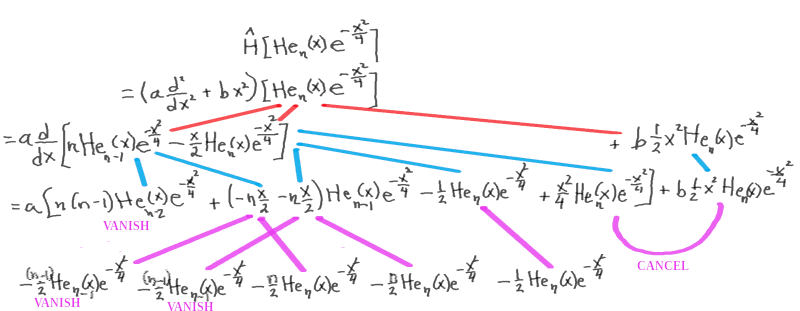
The same calculation in terms of probabilist Hermite polynomials

Our combinatorial interpretation is best made in terms of the probabilist Hermite polynomials and so we need to convert the expressions above.

The physicist Hermite polynomial {$H_n(x)$} is related to the probabilist Hermite polynomial {$\textrm{He}_n(y)$} by the equations {$H_n(x)=2^{\frac{n}{2}}\textrm{He}_n(\sqrt{2}x)$} and {$\textrm{He}_n(y)=2^{-\frac{n}{2}}H_n(\frac{x}{\sqrt{2}})$}.

Instead of {$\psi_n(x) = H_n(\xi)\cdot C_ne^{-\frac{\xi^2}{2}}$} where {$\xi =\sqrt{\frac{m\omega}{\hbar}}x$} we should write {$\psi_n(x) = 2^{\frac{n}{2}}\textrm{He}_n(y)\cdot C_ne^{-\frac{y^2}{4}}$} where {$y =\sqrt{\frac{2m\omega}{\hbar}}x$}.

{$\frac{\partial\textrm{He}_n}{\partial y}=n\textrm{He}_{n-1}(y)$}

{$\hat{H}\psi_n(x) = \frac{-1}{2m}\hbar^2\frac{\partial}{\partial x}\frac{\partial}{\partial x} 2^{\frac{n}{2}}\textrm{He}_n(y)\cdot C_ne^{-\frac{y^2}{4}} + \frac{1}{2m}(m\omega)^2 \frac{\hbar}{m\omega} \frac{1}{2} y^2 2^{\frac{n}{2}}\textrm{He}_n(y)\cdot C_ne^{-\frac{y^2}{4}}$}

{$ = \frac{-1}{2m}\hbar^2\frac{2m\omega}{\hbar}2^{\frac{n}{2}}\frac{\partial}{\partial y}\frac{\partial}{\partial y} \textrm{He}_n(y)\cdot C_ne^{-\frac{y^2}{4}} + \frac{1}{2m}(m\omega)^2 \frac{\hbar}{m\omega}\frac{1}{2} y^2 2^{\frac{n}{2}} \textrm{He}_n(y)\cdot C_ne^{-\frac{y^2}{4}}$}

{$ = -2^{\frac{n}{2}}\hbar\omega\frac{\partial}{\partial y}(n \textrm{He}_{n-1}(y)\cdot C_ne^{-\frac{y^2}{4}} - \textrm{He}_n(y)\cdot \frac{1}{2}y C_ne^{-\frac{y^2}{4}}) + \frac{1}{4}y^2 \textrm{He}_n(y)\cdot \hbar \omega 2^{\frac{n}{2}}C_ne^{-\frac{y^2}{4}}$}

{$ = -2^{\frac{n}{2}}\hbar\omega(n(n-1) \textrm{He}_{n-2}(y)\cdot C_ne^{-\frac{y^2}{4}} - n \textrm{He}_{n-1}(y)\cdot \frac{1}{2} y C_ne^{-\frac{y^2}{4}} - n \textrm{He}_{n-1}(y)\cdot \frac{1}{2}y C_ne^{-\frac{y^2}{4}} - \textrm{He}_n(y)\cdot \frac{1}{2} C_ne^{-\frac{y^2}{4}} + \textrm{He}_n(y)\cdot \frac{1}{4} y^2 C_ne^{-\frac{y^2}{4}} ) + \frac{1}{4}y^2 \textrm{He}_n(y)\cdot \hbar \omega 2^{\frac{n}{2}} C_ne^{-\frac{y^2}{4}}$}

{$ = -2^{\frac{n}{2}}\hbar\omega (n(n-1) \textrm{He}_{n-2}(y) - ny \textrm{He}_{n-1}(y) + (-\frac{1}{2} + \frac{1}{4}y^2 + -\frac{1}{4}y^2 )\textrm{He}_n(y))C_ne^{-\frac{y^2}{4}} $}

{$ = -2^{\frac{n}{2}}\hbar\omega (n(n-1) \textrm{He}_{n-2}(y) - ny \textrm{He}_{n-1}(y) - \frac{1}{2}\textrm{He}_n(y))C_ne^{-\frac{y^2}{2}} $} and make use of the recursion relation {$\textrm{He}_{n+1}(y)=y \textrm{He}_n(y) - n \textrm{He}_{n-1}(y)$} to identify {$n y \textrm{He}_{n-1}(y)= n \textrm{He}_{n}(y) + n^2 \textrm{He}_{n-2}(y)$}.

{$ = -2^{\frac{n}{2}}\hbar\omega (n(n-1) \textrm{He}_{n-2}(y) - n \textrm{He}_{n}(y) - n^2 \textrm{He}_{n-2}(y) - \frac{1}{2}\textrm{He}_n(y))C_ne^{-\frac{y^2}{4}} $}

{$ = -2^{\frac{n}{2}}\hbar\omega (-n\textrm{He}_{n-2}(y) - (n+\frac{1}{2}) \textrm{He}_n(y))C_ne^{-\frac{y^2}{4}} $}

Then by orthogonality

{$\langle H\rangle =\int\psi^*\hat{H}\psi dx = \int 2^{\frac{n}{2}} \textrm{He}_n(y)\cdot C_ne^{-\frac{y^2}{4}}(-2^{\frac{n}{2}})\hbar\omega (-n \textrm{He}_{n-2}(y) - (n+\frac{1}{2}) \textrm{He}_n(y))C_ne^{-\frac{y^2}{4}} dx$}

{$ = -2^n\int \textrm{He}_n(\xi)\cdot C_ne^{-\frac{y^2}{4}}\hbar\omega (-n \textrm{He}_{n-2}(y) - (n+\frac{1}{2}) \textrm{He}_n(y))C_ne^{-\frac{y^2}{4}} \sqrt{\frac{\hbar}{2m\omega}}dy$}

{$= (n+\frac{1}{2})2^n\hbar\omega \sqrt{\frac{\hbar}{2m\omega}} C_n^2 \int \textrm{He}_n(y) \textrm{He}_n(y) e^{-\frac{y^2}{2}} dy $}

{$= (n+\frac{1}{2})2^n\hbar\omega \sqrt{\frac{\hbar}{2m\omega}} (\frac{m\omega}{\pi\hbar})^{\frac{1}{2}}\frac{1}{2^nn!} \int_{-\infty}^{\infty} \textrm{He}_n(y) \textrm{He}_n(y) C_ne^{-\frac{y^2}{2}} dy $} and the integral by orthogonality yields the factor n!{$\sqrt{2\pi}$}

{$= (n+\frac{1}{2})\hbar\omega\frac{1}{\sqrt{2\pi}}\frac{1}{n!}n!\sqrt{2\pi}$}

{$= (n+\frac{1}{2})\hbar\omega$} as required.

Explain the combinatorics of the Hamiltonian in terms of the combinatorics of differentiation and multiplication.

Investigation: Calculate {$\langle H\rangle$} in the general case for {$\psi=\sum_{n=0}^{\infty}c_n\psi_n$}.

I start with the equation for the orthogonality of the monic Sheffer polynomial {$P_n(x)$} as given by Kim and Zeng. In my notation:

{$\mathcal{L}(P_n(x)P_n(x))=n!(c)_n\alpha^n\beta^n$}

Note that if {$c$} in an integer, then {$(c)_n=\frac{c!}{(c-n)!}$}. Note also that this is the monic case, and that the Meixner polynomials are not monic, so I will need to convert them.

Meixner case

The distribution for the Meixner polynomials is {$\omega(x)=\left(\frac{\alpha}{\beta}\right)^n\frac{(c)_n}{n!}$} at {$x=(\alpha-\beta)n\;\;\;n=0,1,2,\dots$}. Equivalently, if {$c$} is an integer, this is: {$\left(\frac{\alpha}{\beta}\right)^n\binom{c}{n}$}.

We integrate across this distribution from {$n(\alpha - \beta)$} to {$(n+1)(\alpha - \beta)$} by simply multiplying by {$\alpha - \beta$} to get the area under the step function.

The probability {$p(n)$} that a particle whose state is given by {$P_k(x)$} is in the interval {$[n(\alpha - \beta), (n+1)(\alpha - \beta))$} is given by:

{$p_k(n(\alpha - \beta))=P_k(n(\alpha - \beta))^2\left(\frac{\alpha}{\beta}\right)^n\binom{c}{n}(\alpha - \beta)$}

The orthogonality relation is given by

{$\sum_{x=0}^{\infty}m_n(x;c,\frac{\alpha}{\beta})m_p(x;c,\frac{\alpha}{\beta})\frac{(\frac{\alpha}{\beta})^x(c)_x}{x!}=(\frac{\beta}{\beta-\alpha})^c(\frac{\beta}{\alpha})^nn!(c)_n\delta_{np}$}

We need to convert this to Kim and Zeng's notation for the monic version of the polynomial {$P_n(x)$} where {$m_n(x;c,\frac{\alpha}{\beta})=\frac{1}{\alpha^n}P_n((\alpha-\beta)x)$}

{$\sum_{x=0}^{\infty}\frac{1}{\alpha^{2n}}P_n((\alpha - \beta)x)^2\frac{(c)_x}{x!}(\frac{\alpha}{\beta})^x = (\frac{\beta}{\beta - \alpha})^c (\frac{\beta}{\alpha})^n n!(c)_n$}

{$(\frac{\beta - \alpha}{\beta})^c \sum_{x=0}^{\infty}P_n((\alpha - \beta)x)^2 \frac{(c)_x}{x!}(\frac{\alpha}{\beta})^x = n!(c)_n \alpha^n \beta^n $}

{$(\frac{\beta - \alpha}{\beta})^c \sum_{\frac{y}{\alpha - \beta}=0}^{\infty} P_n(y)^2 \frac{(c)_{\frac{y}{\alpha - \beta}}} {{\frac{y}{\alpha - \beta}}!}(\frac{\alpha}{\beta})^{\frac{y}{\alpha - \beta}} = n!(c)_n \alpha^n \beta^n $}

So this defines the distribution for the monic Meixner polynomial which Kim and Zeng use in their linearization formula.

It is possible (I need to double check) that each term in the sum is positive. This means that each term gives the probability density of the particle being located there. So we can simply multiply by a small interval {$h$} or I think even {$\alpha - \beta$} to get the probability. Thus the probability density would be:

{$p_n((\alpha - \beta)k) = (\frac{\beta - \alpha}{\beta})^c \frac{1}{n!(c)_n \alpha^n \beta^n}P_n((\alpha - \beta)k)^2 \frac{(c)_k}{k!}(\frac{\alpha}{\beta})^k$}

{$p_n((\alpha - \beta)k) = (1-\frac{\alpha}{\beta})^c \frac{\alpha^{k-n}}{\beta^{k+n}}\binom{c}{n}\binom{c}{k}P_n((\alpha - \beta)k)^2$}

This suggests that {$c$} is a positive integer such that {$c\geq n,k$}. And that {$n$} is the state of evolution in the causal hierarchy and that {$k$} is the state of evolution in the temporal (=distance) sequence.

Note that for the Meixner polynomial distribution, {$x$} is not the typical continual variable from negative infinity to positive infinity. Instead, x is an integer value that is the discrete counting of the unfolding of possibilities, as with time. Which is to say, x is the parameter that indicates the state of a system as it evolves discretely.

Note that if we sum over the entire distribution we should get

{$\sum_{n=0}^{\infty}p_k(n(\alpha - \beta))=\sum_{n=0}^{\infty}P_k(n(\alpha - \beta))^2\left(\frac{\alpha}{\beta}\right)^n\binom{c}{n}(\alpha - \beta) = k!(c)_k\alpha^k\beta^k$}

We can normalize this by dividing. But this is not informative. Instead, we should understand the combinatorial interpretation of orthogonality given by Kim and Zeng.

Another way to proceed is to look at Kim and Zeng's orthogonality formula

{$\mathcal{L}(P_n(x)P_n(x))=n!(c)_n\alpha^n\beta^n$}

and relate that to the formula for the moments (given by permutations) and to the combinatorial expression for the polynomial coefficients (given by pairs of trees) to get the term {$n!(c)_n\alpha^n\beta^n$}.

Hermite case

Subsequently, I will attempt the Hermite case. I need to express that in terms of Hermite polynomials. I need to integrate the square of the polynomials times the weight function, and then express that in terms of {$x+h$} and {$x$} and then subtract. This is related to the Error function.

Tom Leinster. The Categorical Origins Of Entropy.

• https://www.maths.ed.ac.uk/~tl/b.pdf
• Given an operad O and and O-algebra in Cat, there is a general concept of internal algebra in A. Applied to the terminal monad 1, this gives the concept of (internal) monoid in a monoidal category. Applied to the operad Δ of simplices and its algebra (R,+,0) in Cat, it gives the concept of Shannon entropy.
• Given an operad O, we can create the free categorical O-algebra containing an internal algebra. When O=1, this is the category of finite totally ordered sets. When O=Δ, then this is (nearly) the category of finite probability spaces.
• Relate this to Sheffer polynomials.

Jiang Zeng. Weighted Derangements and the Linearization Coefficients of Orthogonal Sheffer Polynomials

• This paper expresses the generating function of the linearization coefficients of all the orthogonal Sheffer polynomials in terms of elementary symmetric functions. I can study what that means for elementary symmetric functions of the eigenvalues of a matrix, especially for the case of the Meixner polynomials.

{$\sum_{n\geq 0}\mathcal{M}(\mathbf{n};\beta,c)\frac{\mathbf{x}^{\mathbf{n}}}{\mathbf{n}!}=\{1-\sum_{k=2}^m(c+\dots +c^{k–1})e_k)^{-\beta}\}$}

Here are key papers that I am studying.

• Paul Butzer. Tom Koornwinder. Josef Meixner: His life and his orthogonal polynomials. 2019. (PDF) Summarizes Meixner's 1934 paper including his derivation of the fivefold classification.
  • Tom Koornwinder. Explanation of steps in the proof!
  • Meixner, Josef. Orthogonale Polynomsysteme mit einer besonderen Gestalt der erzeugenden Funktion, J. London Math. Soc. 9 (1934), 6–13; JFM 60.0293.01; Zbl 0008.16205.
• Isador M. Sheffer. Some properties of polynomial sets of type zero. 1939. A better resolution copy is available at archive.org
• In 1990, J. Zeng, Linearisation de produits de polynomes de Meixner, Krawtchouk, et Charlier, SIAM J.Math. Anal.,21 (1990), 1349–1368.
• In 2001, Dongsu Kim and Jiang Zeng published A Combinatorial Formula for the Linearization Coefficients of General Sheffer Polynomials. Here I found their combinatorial interpretation of the Sheffer polynomials and also their orthogonality equations.
• Francesco Aldo Costabile, Maria Italia Gualtieri, Anna Napoli. Towards the Centenary of Sheffer Polynomial Sequences: Old and Recent Results. 2022.
• Daniel Galiffa, Tanya Riston. An elementary approach to characterizing Sheffer A-type 0 orthogonal polynomial sequences. 2015.
• Carl Morris. Natural Exponential Families with Quadratic Variance Functions. 1982
• Xavier Viennot's website
• The Art of Bijective Combinatorics Part IV. A combinatorial theory of orthogonal polynomials and continued fractions. Chapters 7-10
  • Chapter 5. Orthogonality and exponential structures.
  • Xavier Viennot. Chapter 5c: Tableaux and Orthogonal Polynomials
• Theodore Chihara. An Introduction to Orthogonal Polynomials. 1978. I found this book helpful.

Related pages:

• Meixner polynomials I work out my expressions for the recurrence relation and the Meixner polynomials.
• Sheffer polynomial investigation Most recent attempt to write up what I know.
• Sheffer Polynomials: Combinatorial Space for Quantum Physics My talk on pointed partitions.
• Sheffer classification Wrote out some tasks to do.
• Sheffer polynomials Initial thoughts on the combinatorics and classification of the Sheffer polynomials.
• Feynman diagrams Combinatorics of the Feynman diagrams.
• Moments I looked for the meaning of the weight function.
• Wick's theorem I noticed that the combinatorics was the same as for the Hermite polynomials.
• Orthogonal polynomials Initial study of the combinatorics of solutions to the Schroedinger equation.
• Schroedinger equation My study of the Schroedinger equation led me to the study of the combinatorics of the orthogonal polynomials.