Introduction E9F5FC

Questions FFFFC0

• View
• Edit
• History
• Print

Category theory for statistics would require graded morphisms. Each morphism should have a real number that would give its significance. Thus we could restrict our attention to those morphisms that satisfy a certain significance.

It seems that Bayesian and frequentist interpretations are adjoint functors. One is a prior adjustment (priors) and the other is a post adjustment (replication). So they would be like unit and counit.

Adjoint functors

• Adjoint functors - Tensor product of independent factors - the adjoint functor of this "trivial action" is randomness, the idea that when we don't know, we should assume equal probability.
• Sufficient statistic A statistic is sufficient with respect to a statistical model and its associated unknown parameter if "no other statistic that can be calculated from the same sample provides any additional information as to the value of the parameter".[1] In particular, a statistic is sufficient for a family of probability distributions if the sample from which it is calculated gives no additional information than the statistic, as to which of those probability distributions is the sampling distribution.
• Fisher–Neyman factorization theorem provides a convenient characterization of a sufficient statistic. If the probability density function is {$ƒ_θ(x)$}, then T is sufficient for θ if and only if nonnegative functions g and h can be found such that {$f_{\theta }(x)=h(x)\,g_{\theta }(T(x))$} i.e. the density ƒ can be factored into a product such that one factor, h, does not depend on θ and the other factor, which does depend on θ, depends on x only through T(x).
• Basu's theorem Any boundedly complete minimal sufficient statistic is independent of any ancillary statistic. It is often used in statistics as a tool to prove independence of two statistics, by first demonstrating one is complete sufficient and the other is ancillary, then appealing to the theorem. An example of this is to show that the sample mean and sample variance of a normal distribution are independent statistics. This property (independence of sample mean and sample variance) characterizes normal distributions.
• Akaike information criterion an estimator of in-sample prediction error and thereby relative quality of statistical models for a given set of data. In-sample prediction error is the expected error in predicting the resampled response to a training sample. Given a collection of models for the data, AIC estimates the quality of each model, relative to each of the other models. Thus, AIC provides a means for model selection. If out-of-sample prediction error is expected to differ from in-sample prediction error, cross-validation is a better estimate of model quality. AIC is founded on information theory. When a statistical model is used to represent the process that generated the data, the representation will almost never be exact; so some information will be lost by using the model to represent the process. AIC estimates the relative amount of information lost by a given model: the less information a model loses, the higher the quality of that model. In estimating the amount of information lost by a model, AIC deals with the trade-off between the goodness of fit of the model and the simplicity of the model. In other words, AIC deals with both the risk of overfitting and the risk of underfitting.
• Cross-validation, sometimes called rotation estimation or out-of-sample testing, is any of various similar model validation techniques for assessing how the results of a statistical analysis will generalize to an independent data set. It is mainly used in settings where the goal is prediction, and one wants to estimate how accurately a predictive model will perform in practice. In a prediction problem, a model is usually given a dataset of known data on which training is run (training dataset), and a dataset of unknown data (or first seen data) against which the model is tested (called the validation dataset or testing set). The goal of cross-validation is to test the model's ability to predict new data that was not used in estimating it, in order to flag problems like overfitting or selection bias and to give an insight on how the model will generalize to an independent dataset (i.e., an unknown dataset, for instance from a real problem).
• Bayes factors is a Bayesian alternative to classical hypothesis testing. Bayesian model comparison is a method of model selection based on Bayes factors. The models under consideration are statistical models. The aim of the Bayes factor is to quantify the support for a model over another, regardless of whether these models are correct. The Bayes factor is a likelihood ratio of the marginal likelihood of two competing hypotheses, usually a null and an alternative. When the two models are equally probable a priori, so that {$\Pr(M_{1})=\Pr(M_{2}$}, the Bayes factor is equal to the ratio of the posterior probabilities of {$M_1$} and {$M_2$}. If instead of the Bayes factor integral, the likelihood corresponding to the maximum likelihood estimate of the parameter for each statistical model is used, then the test becomes a classical likelihood-ratio test. Unlike a likelihood-ratio test, this Bayesian model comparison does not depend on any single set of parameters, as it integrates over all parameters in each model (with respect to the respective priors). However, an advantage of the use of Bayes factors is that it automatically, and quite naturally, includes a penalty for including too much model structure.[6] It thus guards against overfitting.
• Can treat model comparison as a decision problem, computing the expected value or cost of each model choice.
• Can compare models by using minimum message length (MML).
• Basu's paradoxes: Reviewed Work: Selected Works of Debabrata Basu by Anirban DasGupta
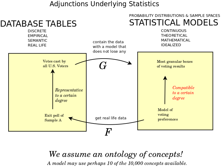
• In returning from database tables to statistical compartments we append all concepts. But we append them as trivial compartments. Such trivial compartments may be understood to have trivial values, which is to say, known values, specific values, ranging over measure zero. They have no meaningful variation.

Bayesian vs. Frequentist

• See also Likelihood approach.
• Bayesian adjusts the model. Frequentist adjusts the observations.
• Christian Bartels Bayesian statistics starts from what has been observed and assesses possible future outcomes. Frequentist statistics starts with an abstract experiment of what would be observed if one assumes something, and only then compares the outcomes of the abstract experiment with what was actually observed. Otherwise the two approaches are compatible. They both assess the probability of future observations based on some observations made or hypothesized.
• Christian Bartels. Positioning Bayesian inference as a particular application of frequentist inference and viceversa
• Bayesian inference derives the posterior probability as a consequence of two antecedents: a prior probability and a "likelihood function" derived from a statistical model for the observed data. Bayesian inference computes the posterior probability according to Bayes' theorem: {$P(H\mid E)={\frac {P(E\mid H)\cdot P(H)}{P(E)}}$}.

Yoneda lemma

• Bayesian inference models statistical inference in terms of steps. Frequentist inference models statistical inference in terms of the whole.

Patterson

• page 4: "statistics first established itself as an independent field in the early twentieth century. Its central concepts are the statistical model, as a parametric family of probabilistic data generating mechanisms, and statistical inference, as the approximate inversion of a statistical model to infer model parameters from observed data. Statistical inference is often classified according to whether it is frequentist or Bayesian and whether it concerns parameter estimation, hypothesis testing, or prediction.
• page 77: "Taking the domain x to be the monoidal unit I recovers the simpler notion of disintegrating a distribution. Bayesian inference can then be formulated in any Markov category in which the required disintegrations exist: given a sampling or likelihood morphism {$p : θ → x$} and a prior {$π_0 : I → θ$}, first integrate with respect to θ to obtain a joint distribution {$I → θ ⊗ x$}, then disintegrate with respect to x to obtain a posterior {$π_1 : x → θ$} and a marginal likelihood {$p_x : I → x$}. Conditional independence and exchangeability can also be formulated in any Markov category."
• page 97: "Statistical theories and models are Bayesian when they are accompanied by a prior. ... Morphisms of Bayesian models, and the category of models of a Bayesian theory, are those of the underlying statistical models and theory. In practice, however, extending a “frequentist” statistical theory (T, p) to a Bayesian one typically requires the category T to be enlarged with another morphism, representing the prior, and this changes the class of models and their morphisms."
• page 108: "In the category of Bayesian statistical theories and (co)lax morphisms, composition and identities are those of the (co)lax morphisms between the underlying statistical theories. Thus, by construction, there is a forgetful functor from the category of Bayesian theories to the category of statistical theories, which discards the prior. Another forgetful functor performs marginalization..." [The adjoint functors are the related constructions...]
• page 110: "Remarkably, Fritz has recently demonstrated that sufficiency, ancillarity, completeness, and minimal sufficiency may be defined, and versions of the Neyman-Fisher factorization theorem, Basu’s theorem, and Bahadur’s theorem proved, in the purely synthetic setting of a Markov category [Fri20]. All of these belong to the classic definitions and abstract results of statistical decision theory"

Concepts related to composition

• Statistical inference (Inferential statistics): Deducing properties of the model. In machine learning, referred to as training or learning.
• Descriptive statistics: Properties of observed data without assuming it comes from a larger population.
• Prediction (Predictive inference): In machine learning, inference: Making a prediction by evaluating an already trained model.

Possible adjoint functors

• In statistics a minimum-variance unbiased estimator (MVUE) or uniformly minimum-variance unbiased estimator (UMVUE) is an unbiased estimator that has lower variance than any other unbiased estimator for all possible values of the parameter. For practical statistics problems, it is important to determine the MVUE if one exists, since less-than-optimal procedures would naturally be avoided, other things being equal. This has led to substantial development of statistical theory related to the problem of optimal estimation. While combining the constraint of unbiasedness with the desirability metric of least variance leads to good results in most practical settings—making MVUE a natural starting point for a broad range of analyses—a targeted specification may perform better for a given problem; thus, MVUE is not always the best stopping point.
• In statistical hypothesis testing, a uniformly most powerful (UMP) test is a hypothesis test which has the greatest power {$1 − β$} among all possible tests of a given size {$α$}.
• The Neyman-Pearson lemma show that the likelihood-ratio test is the most powerful test, among all possible statistical tests.
• The likelihood-ratio test assesses the goodness of fit of two competing statistical models based on the ratio of their likelihoods, specifically one found by maximization over the entire parameter space and another found after imposing some constraint. If the constraint (i.e., the null hypothesis) is supported by the observed data, the two likelihoods should not differ by more than sampling error.[1] Thus the likelihood-ratio test tests whether this ratio is significantly different from one, or equivalently whether its natural logarithm is significantly different from zero.
• The likelihood-ratio test is the oldest of the three classical approaches to hypothesis testing, together with the Lagrange multiplier test and the Wald test.[2] In fact, the latter two can be conceptualized as approximations to the likelihood-ratio test, and are asymptotically equivalent.[3][4][5] In the case of comparing two models each of which has no unknown parameters, use of the likelihood-ratio test can be justified by the Neyman–Pearson lemma. [Are the other two tests the left and right adjoint functors?]
• Loss functions need not be explicitly stated for statistical theorists to prove that a statistical procedure has an optimality property. However, loss-functions are often useful for stating optimality properties: for example, median-unbiased estimators are optimal under absolute value loss functions, in that they minimize expected loss, and least squares estimators are optimal under squared error loss functions, in that they minimize expected loss.
• In mathematical optimization and decision theory, a loss function or cost function is a function that maps an event or values of one or more variables onto a real number intuitively representing some "cost" associated with the event. An optimization problem seeks to minimize a loss function. An objective function is either a loss function or its negative (in specific domains, variously called a reward function, a profit function, a utility function, a fitness function, etc.), in which case it is to be maximized. In statistics, typically a loss function is used for parameter estimation, and the event in question is some function of the difference between estimated and true values for an instance of data. The concept, as old as Laplace, was reintroduced in statistics by Abraham Wald in the middle of the 20th century.[1] In the context of economics, for example, this is usually economic cost or regret. In classification, it is the penalty for an incorrect classification of an example. In actuarial science, it is used in an insurance context to model benefits paid over premiums, particularly since the works of Harald Cramér in the 1920s.[2] In optimal control, the loss is the penalty for failing to achieve a desired value. In financial risk management, the function is mapped to a monetary loss. In classical statistics (both frequentist and Bayesian), a loss function is typically treated as something of a background mathematical convention.
• While statisticians using frequentist inference must choose for themselves the parameters of interest, and the estimators/test statistic to be used, the absence of obviously explicit utilities and prior distributions has helped frequentist procedures to become widely viewed as 'objective'.
• Bayesian inference The Bayesian calculus describes degrees of belief using the 'language' of probability; beliefs are positive, integrate to one, and obey probability axioms. Bayesian inference uses the available posterior beliefs as the basis for making statistical propositions. There are several different justifications for using the Bayesian approach.
• Formally, Bayesian inference is calibrated with reference to an explicitly stated utility, or loss function; the 'Bayes rule' is the one which maximizes expected utility, averaged over the posterior uncertainty. Formal Bayesian inference therefore automatically provides optimal decisions in a decision theoretic sense. Given assumptions, data and utility, Bayesian inference can be made for essentially any problem, although not every statistical inference need have a Bayesian interpretation. Analyses which are not formally Bayesian can be (logically) incoherent; a feature of Bayesian procedures which use proper priors (i.e. those integrable to one) is that they are guaranteed to be coherent.
• Likelihoodism approaches statistics by using the likelihood function. Some likelihoodists reject inference, considering statistics as only computing support from evidence. Others, however, propose inference based on the likelihood function, of which the best-known is maximum likelihood estimation.
• Maximum likelihood estimation (MLE) is a method of estimating the parameters of a probability distribution by maximizing a likelihood function, so that under the assumed statistical model the observed data is most probable. The point in the parameter space that maximizes the likelihood function is called the maximum likelihood estimate. The logic of maximum likelihood is both intuitive and flexible, and as such the method has become a dominant means of statistical inference. From the vantage point of Bayesian inference, MLE is a special case of maximum a posteriori estimation (MAP) that assumes a uniform prior distribution of the parameters. In frequentist inference, MLE is a special case of an extremum estimator, with the objective function being the likelihood.
• Norman Anderson: How to integrate other evidence besides the possibility of chance?
• Frequentist foundation epitomized by sampling distribution, underlies the classical approach to Anova regression. But how to treat unique events?
• The Akaike information criterion (AIC) is an estimator of the relative quality of statistical models for a given set of data. Given a collection of models for the data, AIC estimates the quality of each model, relative to each of the other models. Thus, AIC provides a means for model selection. AIC is founded on information theory: it offers an estimate of the relative information lost when a given model is used to represent the process that generated the data. (In doing so, it deals with the trade-off between the goodness of fit of the model and the simplicity of the model.)
• The minimum description length (MDL) principle has been developed from ideas in information theory[46] and the theory of Kolmogorov complexity.[47] The (MDL) principle selects statistical models that maximally compress the data; inference proceeds without assuming counterfactual or non-falsifiable "data-generating mechanisms" or probability models for the data, as might be done in frequentist or Bayesian approaches. However, if a "data generating mechanism" does exist in reality, then according to Shannon's source coding theorem it provides the MDL description of the data, on average and asymptotically.[48] In minimizing description length (or descriptive complexity), MDL estimation is similar to maximum likelihood estimation and maximum a posteriori estimation (using maximum-entropy Bayesian priors). However, MDL avoids assuming that the underlying probability model is known; the MDL principle can also be applied without assumptions that e.g. the data arose from independent sampling.

Readings

• Wikipedia: Statistical inference
• Inverse-gamma distribution

Notes

• The concepts are less than the number of instances. Because at least the empirical concepts are based on repetition, recurrence.
• Yoneda lemma - do nothing action on models - corresponds to repeating a survey/experiment.
• Indexed functors - graded monoids - statistics. Ross Street, 1972. Graded monads come from graded adjunctions.